Erasure Coding for Distributed Systems
Suppose one has \(N\) servers across which to store a file. One extreme is to give each of the \(N\) servers a full copy of the file. Any server can supply a full copy of the file, so even if \(N-1\) servers are destroyed, then the file hasn’t been lost. This provides the best durability and fault tolerance but is the most expensive in terms of storage space used. The other extreme is to carve the data up into \(N\) equal-sized chunks, and give each server one chunk. Reading the file will require reading all \(N\) chunks and reassembling the file. This will provide the best cost efficiency, as each server can contribute to the file read request while using the minimum amount of storage space.
Erasure codes are the way to more generally describe the space of trade-offs between storage efficiency and fault tolerance. One can say "I’d like this file carved into \(N\) chunks, such that it can still be reconstructed with any \(M\) chunks destroyed", and there’s an erasure code with those parameters which will provide the minimum-sized chunks necessary to meet that goal.
The simplest intuition for there being middle points in this tradeoff is to consider a file replicated across three servers such that reading from any two should be able to yield the whole contents. We can divide the file into two pieces, the first half of the file forms the first chunk (\(A\)) and the second half of the file forms the second chunk (\(B\)). We can then produce a third equal-sized chunk (\(C\)) that’s the exclusive or of the first two (\(A \oplus B = C\)). By reading any two of the three chunks, we can reconstruct the whole file:
Chunks Read |
Reconstruct Via |
|---|---|
\(\{A, B\}\) |
\(A :: B\) |
\(\{A, C\}\) |
\(A :: A \oplus C => A :: (A \oplus (A \oplus B)) => A :: B\) |
\(\{B, C\}\) |
\(B \oplus C :: B => (B \oplus (A \oplus B)) :: B => A :: B\) |
And all erasure codes follow this same pattern of having separate data and parity chunks.
Erasure Coding Basics
Configuring an erasure code revolves around one formula:
| \(k\) |
The number of pieces the data is split into. One must read at least this many chunks in total to be able to reconstruct the value. Each chunk in the resulting erasure code will be \(1/k\) of the size of the original file. |
| \(m\) |
The number of parity chunks to generate. This is the fault tolerance of the code, or the number of reads which can fail to complete. |
| \(n\) |
The total number of chunks that are generated. |
Erasure codes are frequently referred to by their \(k+m\) tuple. It is important to note that the variable names are not consistent across all literature. The only constant is that an erasure code written as \(x+y\) means \(x\) data chunks and \(y\) parity chunks.
Please enjoy a little calculator to show the effects of different \(k\) and \(m\) settings:
Erasure codes are incredibly attractive to storage providers, as they offer a way to fault tolerance at minimal storage overhead. Backblaze B2 runs with \(17+3\), allowing it to tolerate 3 failures using 1.18x the storage space. OVH Cloud uses an \(8+4\) code, allowing it to tolerate 4 failures using 1.5x the storage space. Scaleway uses a \(6+3\) code, tolerating three failures using 1.5x the storage space. "Cloud storage reliability for Big Data applications"[1] pays significant attention to the subject of erasure coding due to the fundamental role it plays in increasing durability for storage providers at a minimal cost of additional storage space. [1]: Rekha Nachiappan, Bahman Javadi, Rodrigo N. Calheiros, and Kenan M. Matawie. 2017. Cloud storage reliability for Big Data applications. J. Netw. Comput. Appl. 97, C (November 2017), 35–47. [scholar]
The main trade-off in erasure coding is a reduction in storage space used at the cost of an increase in requests issued to read data. Rather than issuing one request to read a file-sized chunk from one disk, requests are issued to \(k+m\) disks. Storage systems meant for infrequently accessed data, form ideal targets for erasure coding. Infrequent access means issuing more IO operations per second won’t be a problematic tax, and the storage savings are significant when compared to storing multiple full copies of every file.
"Erasure coding" describes a general class of algorithms and not any one algorithm in particular. In general, Reed-Solomon codes can be used to implement any \(k+m\) configuration of erasure codes. Due to the prevalence of RAID, special attention in erasure coding research has been paid to developing more efficient algorithms specialized for implementing these specific subsets of erasure coding. RAID-0 is \(k+0\) erasure coding. RAID-1 is \(1+m\) erasure coding. RAID-4 and RAID-5 are slightly different variations of \(k+1\) erasure coding. RAID-6 is \(k+2\) erasure coding. Algorithms specifically designed for these cases are mentioned in the implementation section below, but it’s also perfectly fine to not be aware of what exact algorithm is being used to implement the choice of a specific \(k+m\) configuration.
Everything described in this post is about Minimum Distance Separable (MDS) erasure codes, which are only one of many erasure code families. MDS codes provide the quorum-like property that any \(m\) chunks can be used to reconstruct the full value. Other erasure codes take other tradeoffs, where some combinations of less than \(m\) chunks can be used to reconstruct the full value, but other combinations require more than \(m\) chunks. "Erasure Coding in Windows Azure Storage"[2] nicely explains the motivation of why Azure devised Local Reconstruction Codes for their deployment. "SD Codes: Erasure Codes Designed for How Storage Systems Really Fail"[3] pitches specializing an erasure code towards recovering from sector failures, as the most common failure type. Overall, if one has knowledge about the expected pattern of failures, then a coding scheme that allow recovering from expected failures with less than \(m\) chunks, and unexpected failures with more than \(m\) chunks would have a positive expected value.
[2]: Cheng Huang, Huseyin Simitci, Yikang Xu, Aaron Ogus, Brad Calder, Parikshit Gopalan, Jin Li, and Sergey Yekhanin. 2012. Erasure Coding in Windows Azure Storage. In 2012 USENIX Annual Technical Conference (USENIX ATC 12), USENIX Association, Boston, MA, 15–26. [scholar]
[3]: James S. Plank, Mario Blaum, and James L. Hafner. 2013. SD Codes: Erasure Codes Designed for How Storage Systems Really Fail. In 11th USENIX Conference on File and Storage Technologies (FAST 13), USENIX Association, San Jose, CA, 95–104. [scholar]
Applications in Distributed Systems
Space and Tail Latency Improvements
The most direct application is in reducing the storage cost and increasing the durability of data in systems with a known, fixed set of replicas. Think of blob/object storage or NFS storage. A metadata service maps a file path to a server that stores the file. Instead of having 3 replicas storing the full file each, have 15 replicas store the chunks of the (10+5) erasure coded file. Such a coding yields half the total amount of data to store, and more than double the fault tolerance.
More generally, this pattern translates to "instead of storing data across \(X\) servers, consider storing it across \(X+m\) replicas with an \(X+m\) erasure code". Over on Marc Brooker’s blog, this is illustrated using a caching system. Instead of using consistent hashing to identify one of \(k\) cache servers to query, one can use a \(k+m\) erasure code with \(k+m\) cache servers and not have to wait for the \(m\) slowest responses. This provides both a storage space and tail latency improvement.
Again, the space and latency savings do come at a cost, which is an increase in IOPS/QPS, or effectively CPU. In both cases, we’re betting that the limiting resource which determines how many machines or disks we need to buy is storage capacity, and that we can increase our CPU usage to decrease the amount of data that needs to be stored. If the system is already pushing its CPU limits, then erasure coding might not be a cost-saving idea.
Quorum Systems
Consider a quorum system with 5 replicas, where one must read from and write to at least 3 of them, a simple majority. Erasure codes are well matched on the read side, where a \(3+2\) erasure code equally represents that a read may be completed using the results from any 3 of the 5 replicas. Unfortunately, the rule is that writes are allowed to complete as long as they’re received by any 3 replicas, so one could only use a \(1+2\) code, which is exactly the same as writing three copies of the file. Thus, there are no trivial savings to be had by applying erasure coding.
RS-Paxos[4] examined the applicability of erasure codes to Paxos, and similarly concluded that the only advantage is when there’s an overlap between two quorums of more than one replica. A quorum system of 7 replicas, where one must read and write to at least 5 of them would have the same 2 replica fault tolerance, but would be able to apply a \(3+2\) erasure code. In general, with \(N\) replicas and a desired fault tolerance of \(f\), the best one can do with a fixed erasure coding scheme is \((N-2f)+f\). [4]: Shuai Mu, Kang Chen, Yongwei Wu, and Weimin Zheng. 2014. When paxos meets erasure code: reduce network and storage cost in state machine replication. In Proceedings of the 23rd International Symposium on High-Performance Parallel and Distributed Computing (HPDC '14), Association for Computing Machinery, New York, NY, USA, 61–72. [scholar]
HRaft[5] explores that there is a way to get the desired improvement from a simple majority quorum, but adapting the coding to match the number of available replicas. When all 5 replicas are available then we may use a \(3+2\) encoding, when 4 are available then use a \(2+2\) encoding, and when only 3 are available then use a \(1+2\) encoding[6]. Adapting the erasure code to the current replica availability yields our optimal improvement, but comes with a number of drawbacks. Each write is optimistic in guessing the number of replicas that are currently available, and writes must be re-coded and resent to all replicas if one replica unexpectedly doesn’t acknowledge the write. Additionally, one must still provision the system such that a replica storing the full value of every write is possible, so that after two failures, the system running in a \(1+2\) configuration won’t cause unavailability due to lacking disk space or throughput. However, if failures are expected to be rare and will be recovered from quickly, then HRaft’s adaptive encoding scheme will yield significant improvements. [5]: Yulei Jia, Guangping Xu, Chi Wan Sung, Salwa Mostafa, and Yulei Wu. 2022. HRaft: Adaptive Erasure Coded Data Maintenance for Consensus in Distributed Networks. In 2022 IEEE International Parallel and Distributed Processing Symposium (IPDPS), 1316–1326. [scholar] [6]: And just to emphasize again, a \(1+2\) erasure encoding is just 3 full copies of the data. It’s the same as not applying any erasure encoding. The only difference is that it’s promised that only three full copies of the data are generated and sent to replicas.
Usage Basics
For computing erasure codings, there is a mature and standard Jerasure. If on a modern Intel processor, the Intel Intelligent Storage Acceleration Library is a SIMD-optimized library consistently towards the top of the benchmarks.
As an example, we can use pyeclib as a way to get easy access to an erasure coding implementation from python, and apply it to specifically to HRaft’s proposed adaptive erasure coding scheme:
Python source code
#!/usr/bin/env python
# Usage: ./ec.py <K> <M>
import sys
K = int(sys.argv[1])
M = int(sys.argv[2])

# Requires running the following to install dependencies:
# $ pip install --user pyeclib
# $ sudo dnf install liberasurecode-devel
import pyeclib.ec_iface as ec

# liberasurecode_rs_vand is built into liberasurecode, so this
# shouldn't have any other dependencies.
driver = ec.ECDriver(ec_type='liberasurecode_rs_vand',
                     k=K, m=M, chksum_type='none')
data = bytes([i % 100 + 32 for i in range(10000)])
print(f"Erasure Code(K data chunks = {K}, M parity chunks = {M})"
      f" of {len(data)} bytes")

# Produce the coded chunks.
chunks = driver.encode(data)

# There's some metdata that's prefixed onto each chunk to identify
# its position.  This isn't technically required, but there isn't
# an easy way to disable it.  There's also some additional bytes
# which I can't account for.
metadata_size = len(driver.get_metadata(chunks[0]))
chunk_size = len(chunks[0]) - metadata_size
print(f"Encoded into {len(chunks)} chunks of {chunk_size} bytes")
print("")

# This replication scheme is X% less efficient than writing 1 copy
no_ec_size = (K+M) * len(data)
print(f"No EC: {(M+K)*len(data)} bytes, {1/(K+M) * 100}% efficiency")
print(f"Expected: {(M+K)/K * len(data)} bytes,"
      f" {1/ (1/K * (K+M)) * 100}% efficiency")
total_ec_size = chunk_size * len(chunks)
print(f"Actual: {total_ec_size} bytes,"
      f" {len(data) / total_ec_size * 100}% efficiency")

# Validate that our encoded data decodes using minimal chunks
import random
indexes = random.sample(range(K+M), K)
# Prepended metadata is used to determine the chunk part number
# from the data itself.  Other libraries require this to be
# passed in as part of the decode call.
decoded_data = driver.decode([chunks[idx] for idx in indexes])
assert decoded_data == data
When there are 5/5 replicas available, HRaft would use a \(3+2\) erasure code:
$ ./ec.py 3 2
Erasure Code(K data chunks = 3, M parity chunks = 2) of 10000 bytes
Encoded into 5 chunks of 3355 bytes

No EC: 50000 bytes, 20% efficiency
Expected: 16666.666666666668 bytes, 60.00000000000001% efficiency
Actual: 16775 bytes, 59.61251862891207% efficiency
When there are 4/5 replicas available, HRaft would use a \(2+2\) erasure code:
$ ./ec.py 2 2
Erasure Code(K data chunks = 2, M parity chunks = 2) of 10000 bytes
Encoded into 4 chunks of 5021 bytes

No EC: 40000 bytes, 25% efficiency
Expected: 20000.0 bytes, 50% efficiency
Actual: 20084 bytes, 49.790878311093406% efficiency
When there are 3/5 replicas available, HRaft would use a \(1+2\) erasure code:
$ ./ec.py 1 2
Erasure Code(K data chunks = 1, M parity chunks = 2) of 10000 bytes
Encoded into 3 chunks of 10021 bytes

No EC: 30000 bytes, 33.33333333333333% efficiency
Expected: 30000.0 bytes, 33.33333333333333% efficiency
Actual: 30063 bytes, 33.263480025280245% efficiency
Usage Not So Basics
As always, things aren’t quite perfectly simple.
Decoding Cost Variability
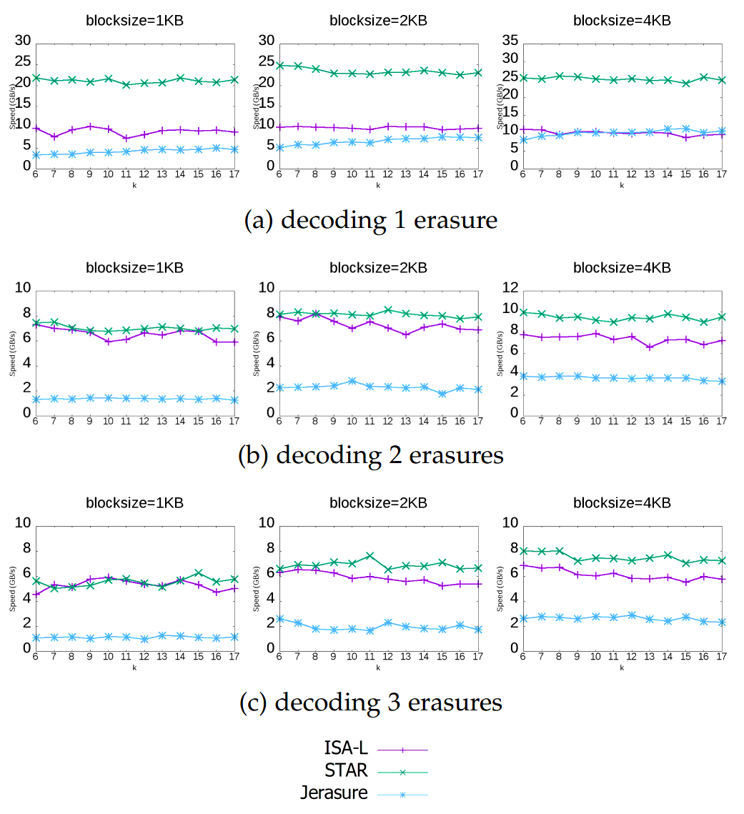
Decoding performance varies with the number of data chunks that need to be recovered. Decoding a \(3+2\) code from the three data chunks is computationally trivial. Decoding the same file from two data chunks and one parity chunk involves solving a system of linear equations via Gaussian elimination, and the computational increases as the number of required parity chunks involved increases. Thus, if using an erasure code as part of a quorum system, be aware that the CPU cost of decoding will vary depending on exactly which replicas reply.
There are a few different papers comparing different erasure code implementations and their performance across varying block size and number of data chunks to reconstruct. I’ll suggest "Practical Performance Evaluation of Space Optimal Erasure Codes for High Speed Data Storage Systems"[7] as the one I liked the most, from which the following figure was taken: [7]: Rui Chen and Lihao Xu. 2019. Practical Performance Evaluation of Space Optimal Erasure Codes for High-Speed Data Storage Systems. SN Comput. Sci. 1, 1 (December 2019). [scholar]
Library Differences
Liberasurecode abstracts over most common erasure coding implementation libraries, but be aware that does not mean that the implementations are equivalent. Just because two erasure codes are both \(3+2\) codes doesn’t mean the same math was used to construct them.
Correspondingly, liberasurecode doesn’t just do the linear algebra work, it "helpfully" adds metadata necessary to configure which decoder to use and how, which you can’t disable or modify:
struct __attribute__((__packed__))
fragment_metadata
{
    uint32_t    idx;                /* 4 */
    uint32_t    size;               /* 4 */
    uint32_t    frag_backend_metadata_size;    /* 4 */
    uint64_t    orig_data_size;     /* 8 */
    uint8_t     chksum_type;        /* 1 */
    uint32_t    chksum[LIBERASURECODE_MAX_CHECKSUM_LEN]; /* 32 */
    uint8_t     chksum_mismatch;    /* 1 */
    uint8_t     backend_id;         /* 1 */
    uint32_t    backend_version;    /* 4 */
} fragment_metadata_t;
This is just a liberasurecode thing. Using either Jerasure or ISA-L directly allows access to only the erasure coded data. It is required as part of the APIs that each chunk must be provided along with if it was the Nth data or parity chunk, so the index must be maintained somehow as part of metadata.
As was noted in the YDB talk at HydraConf, Jerasure does a permutation of the output from what one would expect from just the linear algebra. This means that it’s up to the specific implementation details of a library as to if reads must be aligned with writes — Jerasure cannot read a subset or superset of what was encoded. ISA-L applies no permutation, so reads may decode unaligned subsets or supersets of encoded data.
Jerasure and ISA-L are, by far, the most popular libraries for erasure coding, but they’re not the only ones. tahoe-lafs/zfec is also a reasonably well-known implementation. Christopher Taylor has written at least three MDS erasure coding implementations taking different tradeoffs (catid/cm256
, catid/longhair
, catid/leopard
), and a comparison and discussion of the differences can be found on leopard’s benchmarking results page. If erasure coding becomes a bottleneck, a library more optimized for your specific use case can likely be found somewhere, but ISA-L is generally good enough.
Implementing Erasure Codes
It is entirely acceptable and workable to treat erasure codes as a magic function that turns 1 file into \(n\) chunks and back. You can stop reading here, and not knowing the details of what math is being performed will not hinder your ability to leverage erasure codes to great effect in distributed systems or databases. (And if you continue, take what follows with a large grain of salt, as efficient erasure coding is a subject folk have spent years on, and the below is what I’ve collected from a couple of days of reading through papers I only half understand.)
The construction of the \(n\) chunks is some linear algebra generally involving a Galois Field, none of which is important to understand to be able to productively use erasure codes. Backblaze published a very basic introduction. The best introduction to the linear algebra of erasure coding that I’ve seen is Fred Akalin’s "A Gentle Introduction to Erasure Codes". Reed-Solomon Error Correcting Codes from the Bottom Up covers Reed-Solomon codes and Galois Field polynomials specifically. NASA has an old Tutorial on Reed-Solomon Error Correction Coding. There’s also a plethora of erasure coding-related questions on the Stack Overflow family of sites, so any question over the math that one might have has already likely been asked and answered there.
With the basics in place, there are two main dimensions to investigate: what is the exact MDS encoding and decoding algorithm to implement, and how can one implement that algorithm most efficiently?
Algorithmic Efficiency
In general, most MDS codes are calculated as a matrix multiplication, where addition is replaced with XOR, and multiply is replaced with a more expensive multiplication over GF(256). For the special cases of 1-3 parity chunks (\(m \in \{1,2,3\}\)), there are algorithms not derived from Reed-Solomon and which use only XORs:
-
\(m=1\) is a trivial case of a single parity chunk, which is just the XOR of all data chunks.
-
\(m=2\) is also known as RAID-6, for which I would recommend Liberation codes[8][9] as nearly optimal with an implementation available as part of Jerasure, and HDP codes[10] and EVENODD[11] as notable but patented. If \(k+m+2\) is prime, then X-Codes[12] are also optimal.
Otherwise and more generally, a form of Reed-Solomon coding is used. The encoding/decoding matrix is either a \(k \times n\) Vandermonde[14] matrix with the upper \(k \times k\) of it Gaussian eliminated to form an identity matrix, or an \(k \times k\) identity matrix with a \(k \times m\) Cauchy[15] matrix glued onto the bottom. In both cases, the goal is to form a matrix where the top \(k \times k\) is an identity matrix (so that each data chunk is preserved), and any deletion of \(m\) rows yields an invertible matrix. Encoding is multiplying by this matrix, and decoding deletes the rows corresponding to erased chunks, and then solves the matrix as a system of linear equations for the missing data.
Gaussian elimination, as used in ISA-L, is the simplest method of decoding, but also the slowest. For Cauchy matrixes, this can be improved[16], as done in catid/cm256. The current fastest methods appear to be implemented in catid/leopard
, which uses Fast Fourier Transforms[17][18] for encoding and decoding.
Implementation Efficiency
There are levels of implementation efficiency for erasure codes that function over any \(k+m\) configuration:
-
Implement the algorithm in C, and rely on the compiler for auto-vectorization.
This provides the most straightforward and most portable implementation, at acceptable performance. Usage of
restrictand ensuring the appropriate architecture-specific compilation flags have been specified (e.g.-march=native). -
Rely on a vectorization library or compiler intrinsics to abstract the platform specifics.
google/highway
and xtensor-stack/xsimd
std::experimental::simd. C/C++ compilers also offer builtins for vectorization support.The core of encoding and decoding is Galois field multiply and addition. Optimized libraries for this can be found at catid/gf256
-
Handwrite a vectorized implementation of the core encoding and decoding functions.
Further discussion of fast GF(256) operations can be found in the PARPAR project: fast-gf-multiplication and the xor_depends work. The consensus appears to be that a XOR-only GF multiply should be faster than a table-driven multiply.
Optimizing further involves specializing the code to one specific \(k+m\) configuration by transforming the matrix multiplication with a constant into a linear series of instructions, and then:
-
Find an optimal coding matrix and XOR schedule for the specific GF polynomial and encoding matrix.
-
Apply further operation, memory, and cache optimizations.
The code is publicly available at yuezato/xorslp_ec
-
Programmatically explore an optimized instruction schedule for a specific architecture.
The code is publicly available at Thesys-lab/tvm-ec
For a more fully explored treatment of this topic, please see "Fast Erasure Coding for Data Storage: A Comprehensive Study of the Acceleration Techniques"[19], which also has a video of the presenter if that’s your preferred medium. [19]: Tianli Zhou and Chao Tian. 2020. Fast Erasure Coding for Data Storage: A Comprehensive Study of the Acceleration Techniques. ACM Trans. Storage 16, 1 (March 2020). [scholar]
References
And if you’re looking to broadly dive deeper, I’d suggest starting with reviewing James S. Plank’s publications.
See discussion of this page on Reddit, Hacker News, and Lobsters.